Expertise:
Beginner
Functional Principal Component Analysis
We might now ask what modes of variation we can find in the data. Classical principal components analysis
seeks to reduce the essential dimensionality of a multivariate dataset into independent linear combinations
of the variables. Functional principal components also seeks to reduce the dimensionality of a
functional dataset - by finding those curves, or "harmonics", which capture the essential modes of variation
of the data.
The best way to visualize the results of functional PCA is through plots such as is shown here. The
overall mean curve is plotted in each subplot, along with the "harmonic effects" - that is, the mean curve
plus and minus a multiple of each harmonic curve. This helps clarify the effects of each harmonic on a
typical curve.
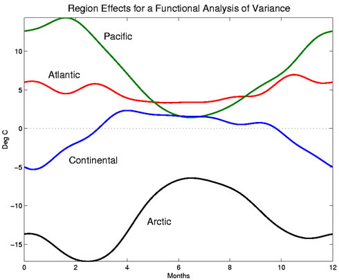
Figure 1: The effects of each region on the temperature functions. These are taken from a
functional
analysis of variance (fANOVA) model described below.
Note that all effects are constrained to sum to 0 for all t.
For instance, here we can see that the first harmonic corresponds to a difference in winter temperatures.
Cities with a high score on this harmonic, for example, would have winters which are consistently
warmer than that of most cities; the Pacific Coast cities are an example of this. This effect accounts
for a large amount of variation in the data - over 89%. The second harmonic, accounting for 8% of
the variation, describes the degree of contrast in winter and summer temperatures. Pacific Coast cities
would again score high on this harmonic, since their winters and summers are more similar to each other
than are most Canadian cities. The third harmonic corresponds to a time shift effect, combined with an
overall increase in temperature and in range between winter and summer. And the fourth corresponds to
an effect in which spring begins later and autumn ends earlier.
Functional Analysis of Variance
Now we ask how much the pattern of annual variation of temperature is attributable to geographic area
- Atlantic, Pacific, Continental, or Arctic. A linear model, or analysis of variance (ANOVA) is a natural
way to quantify these effects. Temperature - a functional observation - is our dependent variable, so we
adapt the classical methodology to create a functional linear model or a fANOVA.
For the ith weather station in the kth climate group, the equation
for this linear model is Tempik(t) = μ(t)
+ αik(t) + εik(t).
Here the αk are the specific effects on temperature of being in
climate group k. We also have a constraint to ensure that the effects are uniquely
identifiable: ∑k αk
(t) = 0 for all t.
This is just like a classical ANOVA model, except the response is a function of time, and so the main
effects α are also functions of time.
The functional effects and fitted values of the functional ANOVA are plotted here, and we can see subtle
effects of the climate on the temperature functions - some of which will be immediately recognizable to
Canadians from their years of personal experience!
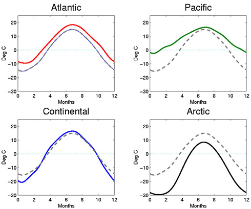
Figure 2: The solid curves are the estimated temperature functions μ(t)
+ αk(t) for the functional
analysis of variance model. The dashed curve is the mean temperature function μ(t).
The Atlantic effect is a nearly constant 5 degrees C across the year, which indicates the Atlantic
stations have a temperature about 5 degrees C warmer year-round than the Canadian average. The Pacific effect is the most variable, with a smaller effect in the summer than in the winter
months. That is, the Pacific weather stations have a summer temperature close to the Canadian
average, but they are much warmer in the winter. The Continental effect is most pronounced in the winter months; these stations are colder than the
average in the winter and only slightly warmer than average in the summer. The Arctic effect is markedly negative, as is expected. The Arctic stations are colder than the
average - but even more so in March than December.
|