Expertise:
Intermediate
What is a spline function?
We need to know what the essential characteristics of splines are before we
consider how to construct a basis system for them.
Spline functions are formed by joining polynomials together at fixed points
called knots. That is, we divide the interval extending from lower limit tL to
upper limit tU over which we wish to approximate a curve into L+1 sub-intervals
separated by L interior boundaries ξl called knots, or sometimes breakpoints.)
There is a distinction between these two terms, but we will come to this later.
Consider the simplest case in which a single breakpoint divides interval
[tL; tU] into two subintervals. The spline
function is, within each interval, a polynomial of specified degree
(the highest power defining the polynomial) or order (the number of
coefficients defining the polynomial, which is one more
than its degree). Let's use m to designate the order of the polynomial,
so that the degree is m - 1:
At the interior breakpoint ξ1, the two
polynomials are required to join smoothly. In the most common case,
this means that the derivatives match up to the order one less than
the degree. In fact, if they matched up to the derivative whose order
equaled the degree, they would be the same polynomial. Thus, a spline
function defined in this was has one extra degree of freedom than
a polynomial extending over the entire interval.
For example, let each polynomial be a straight line segment, and
therefore of degree one. In this, they join at the breakpoint with matching
derivatives
up to degree 0; in short, they simply join and having identical values
at the break point. Since the first polynomial has two degree of freedom (slope
and intercept), and the second, having its value already defined at the
break point, is left with only one degree of freedom (slope), the total polygonal line has three
degrees of freedom.
Correspondingly, if both polynomials are quadratics, then the match both in terms of values and in terms of
slope of first derivative
at ξ1. The first polynomial has three degrees of freedom, but the
second loses two because if the constraint on its value and slope at ξi, and thus retains only
one. This leaves a total of four degrees of freedom for the spline
function formed in this way, as
opposed to three for a quadratic polynomial over the entire interval
[tL; tU]. Figure 1 shows these
linear and quadratic cases with a single breakpoint.
What are some examples of commonly used basis functions?
We can now generalize the situation to L interior breakpoints, and
a spline function being of order m or degree m - 1 over each
sub-interval. The first polynomial segment has a full complement
of m degrees of freedom, but each subsequent segment has only one
degree of freedom because of the m - 1 constraints on its behavior.
This gives a total of L + m degrees of freedom, or number of
interior breakpoints plus the order of the polynomial segments.
Thus, spline functions are essentially generalizations of the notion of polygonal
lines. They gain their flexibility in two ways: First, by the order of the
polynomials from which they are built, and second, by the number of breakpoints
used. We usually elect to keep the order fixed, and add breakpoints as
needed to get the required flexibility.
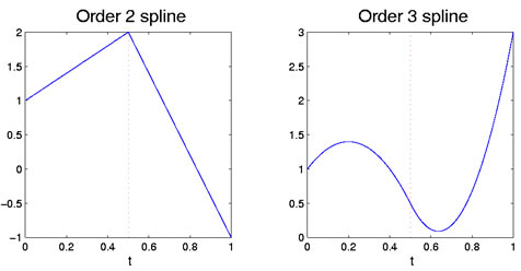
Figure 1: The left figure shows an order two spline function, which
is piecewise linear. The right figure is an order 3 spline, which
is piecewise quadratic. The breakpoint at 0.5 is indicated by the red vertical dotted line.
|