Expertise:
Intermediate
Smoothing with a fourth order roughness penalty
The process generating the data is essentially smooth since the amount of the
data upon which it is based precludes abrupt changes in value. we can exploit
this smoothness by making use of one or more derivatives in our explorations.
In fact, we will find that both the rate of change or velocity and the curvature
or acceleration of the index are useful, and this implies that we should have a
smooth estimate of acceleration.
We choose B-spline basis functions as our basis function system. Why? We
don't use Fourier series here because we don't want to assume the stationarity
of seasonal trend that is built into this basis. On the other hand, B-spline basis
functions are sufficiently flexible to be able to capture both the long-term and
seasonal trends that interest us. Moreover, we can ensure a smooth second
derivative by specifying the order of the spline (the degree plus one of the piecewise
polynomials from which a B-spline basis function is constructed) to be
eight. A knot was placed at each data point. The fitting criterion is
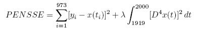
where D4x(t) means the fourth derivative of function x
at time t. We liked the results for smoothing parameter λ = 10-11
since the data points were fit to our satisfaction and the second derivative
curve was smooth.
A bit of jargon: When the order of the spline is twice the order of the
derivative being penalized, and a knot is placed at each data point, we call the
fitted spline function a smoothing spline.
And a computational note: This spline is defined by 977 basis functions,
namely the number of interior knots plus the order. Without some special
computational technology, solving the set of linear equations of order 977 would
challenge the resources most small computers and try the patience of the data
analyst. In Matlab, however, there is the possibility of doing computation in
sparse matrix mode, and most of the elements in the coefficient matrix are zero
because of its banded structure. In S-PLUS, on the other hand, the computation
had to be coded in C to take advantage of the banded structure, and this code
is called by S-PLUS function smooth.Pspline.
|