Expertise:
Intermediate
What is the general idea?
Here is an overview of how we will proceed to construct spline basis functions.
In fact, this is how most basis function systems are constructed.
First we begin with the simplest possible prototype for a basis function.
We call this prototype a mother function, Φ(t). This is our simplest
Lego block, as it were. Next, we apply three operations to the mother function:
Lateral Shift: We displace the mother function along the t axis,
often by defining the displaced version to be Φ(t - δ), where δ is
the amount of the shift. This operation essentially moves fitting
power to where we need it.
Scale change: We change the concentration or lateral variation of the
mother function, or a shifted version of it, by rescaling t to obtain Φ(βt).
The operations can be combined into linear transformations of t to
obtain
Φ(β(t - δ)).
Smoothing: We operate on the mother function to increase its differentiability.
This is the most sophisticated of the three operations.
The shift and scale operations are too simple to require further comment at
this point, but we now need to focus on how spline functions are made more smooth.
How does this smoothing operation work?
First, let the mother basis function be just about the simplest function that
we can imagine, aside perhaps from the constant function. This is the unit
box function, defined as Φ(t) = 1 if 0 ≤ t < 1, and 0 everywhere else. This
is a primitive type of spline function, and is of order 1 or degree 0. It has no
smoothness whatever. See Figure 1 for the mother box function and a laterally
shifted version.
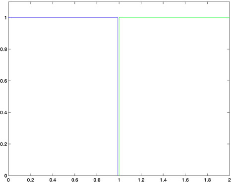
Figure 1: Two box functions. The blue box is the mother basis spline function
of order 1,
and the green is the result of shifting it to the right by one unit.
Now let's apply a tilt to the mother box function by multiplying it
by the function whose value is t if 0 ≤ t, and 0 if t
< 0. The result will be the right triangle function TL(t) = t,
0 ≤ t < 1, and 0
elsewhere. Note that the right triangle will be on the right side of the function,
and the vertical side is positioned over 1.
At the same time, we shift the original box function one unit to the right to
obtain
Φ(t - 1) = 1, 1 ≤ t < 2 and 0 elsewhere.
Moreover, let's then tilt this box, but this time on its right instead
of its left, by multiplying it by 2 - t, t ≤ 2.
The result is also a right triangle, but this time with the right angle on the left
instead of the right, and and its vertical is also positioned over 1.
Finally, we add these two triangle functions together. The result
is the tent or hat function, shown in the bottom panel of Figure 2, that is 0 at
and below t = 0, 0 at and above t = 2, rises linearly to 1 at t =
1, and then declines linearly to 0 at t = 2. What we have achieved
is now a slightly less primitive spline. It has smoothness of order 2 or degree
1 since the two line segments that define it join at the single breakpoint at t = 1.
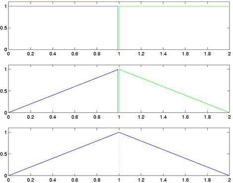
Figure 2: The top panel shows the mother box function Φ(t) in blue, and a
right-displaced version Φ(t - 1) in green.
The center panel shows the two box
functions in top panel tilted, the blue one from the left, and
the green one from
the right. The lower panel shows the sum of these two functions.
This is the
tent function, and is the mother basis spline function of order 2.
Figure 2 shows this process. The center panel shows the blue mother box
function in Figure 1 tilted from the left, and the laterally shifted green box in
Figure 1 tilted from the right. The lower panel shows the tent function resulting
from adding these two tilted functions together. This tent function is the mother
basis spline function of order 2.
|