Expertise:
Beginner
How do I define my B-spline basis?
Two features must be specified. First, because B-splines are polynomial segments joined smoothly
together, we must describe the degree of the polynomials
segments, or, equivalently, their order = degree + 1. A good
bet is to choose the order to be at least four larger than the highest
order of derivative that you will need to look at. Here we will
need to look at acceleration, or the second derivative, so we go
with order 6, meaning that the B-splines are piecewise fifth degree
polynomials.
The second feature is a set of points called knots at which
the these polynomials join. The first knot should be at or below
the lowest age (one year old), and the last at or above the largest
age (eighteen years old). The number of knots in between these plot
the order determines the total number of basis functions.
To keep things simple here, we will use the ages of observation
themselves as knots. There are 31 ages, so the total number of B-spline
basis functions is 29 + 6 = 35. In or Matlab software, the basis
system is defined by the single command
hgtbasis = create_bspline_basis([1,18], 35, 6, age);
Sounds good. What's next?
Now we can input the raw height measurements, the ages at which
we made them, and the definition of the basis system into a function
that computes the linear combination of the basis functions that
best fits the data for each child. We organize our raw height measurements
into a table with rows corresponding to ages of measurement, and
columns corresponding to girls Here is a Matlab statement that does
this for height measurements in a matrix hgtfmat:
hgtffd = data2fd(hgtfmat, age, hgtbasis);
The results are shown in Figure 1 for the first girl using the Matlab
command
plotfit_fd(hgtfmat, age, hgtffd);
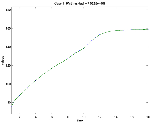
Figure 1: The height of the first girl in the Berkeley Growth Study.
Dots indicate the ages at which measurements were taken.
The title indicates that the typical fitting error is about 0.0000007cm.
No attempt is made here to deal with measurement error.
|