Expertise:
Beginner
How do I actually do this? - Continued
The results are much more interesting when we look at the velocity curves
after smoothing in Figure 3. The Matlab command to do this is
plot(hgtffd, int2Lfd(1))
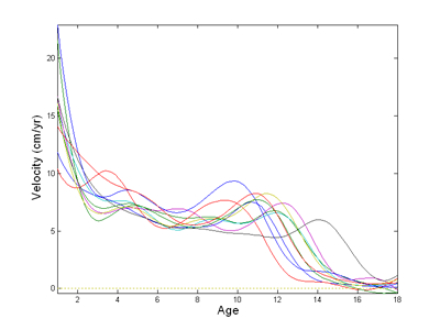
Figure 3: The height velocities of the first 10 girls in the Berkeley Growth Study
after penalizing roughness at the level of the fourth derivative.
Now the velocities seem acceptably smooth, and we can easily note some of
the important characteristics of growth velocity. The pubertal growth spurt is
visible towards the right as a peak in velocity with a maximum of from five to
ten centimeters per year. The timing of this peak varies a lot from girl to girl,
ranging in this plot from ten to fourteen years of age. We also see at least one
earlier smaller peak for most of these curves. But of course the highest velocities
are achieved between one and two years, where they range up to an impressive
25 centimeters per year.
Now we can also look at the acceleration curves with Matlab command
plot(hgtffd, int2Lfd(2)). Although we have to admit that the early accelerations
are pretty wild, we can still see a lot of consistent features in the curves
from six years of age on. The pubertal growth spurt is visible as a peak followed
by a valley, and likewise for the earlier spurts.
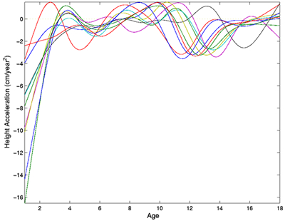
Figure 4: The height accelerations of the first 10 girls in the Berkeley Growth
Study after penalizing roughness at the level of the fourth derivative.
|