Expertise:
Intermediate
How do I choose the order m of a spline?
The most common type of spline is the cubic spline in which
each polynomial is a cubic, or of order 4. Because the segments
join with matching derivatives up
to order 2, they appear to the eye to be beautifully smooth. This
is because the second derivative measure the curvature of a curve,
and the curvatures match
at the breakpoints, so that the curvature appears to change smoothly.
However, the order m that we use depends on how many derivatives we will
need to compute from the spline function. A cubic spline is smooth in itself,
but its first derivative will appear to change with noticeable abruptness at the
breakpoints, and its second derivative will be a polygonal line. What this means
is that if we want a smooth second derivative, we had better use a spline of order
at least six, so that its second derivative will be at least smooth as a cubic spline.
How do I choose the breakpoints ξl?
The more breakpoints, the more flexible the spline. Moreover, this principle
applies locally; if we need a lot of flexibility in a particular region of t,
we use more breakpoints in this region. And, of course, less where we don't need
much curvature.
However, it is pointless to have breakpoints without data. There should in
most situations be at least one observed value ti within each subinterval. If if
one suspects that there is a sharp feature in a particular region, only one or two
data values in its vicinity will pretty much eliminate any hope of adequately
describing it, and the fitted curve may as well be smooth.
The problem of deciding exactly where to position breakpoints is often finessed
in one of two ways. First, users often just make them equally spaced, but
of course paying attention to the requirement of having at least one observation
in every subinterval. The second strategy is the place a breakpoint at every fixed
number of observed values of t, sometimes called quantile placement. This has
the advantage of ensuring that there is a reasonable amount of data associated
with each subinterval.
Figure 2 shows a typical situation in which some discrete noisy data are fit
by a cubic spline function. The breakpoints are as shown, and they are spaced
closer together in the middle where there is obvious more curvature needed than
at the extremes.
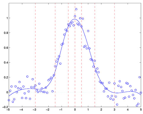
Figure 2: The fit to some discrete noisy data, indicated by circles,
achieved by a cubic spline
function defined by the breakpoint values indicated by the vertical
red dashed lines.
What about spline basis functions?
This discussion only gives a vague idea of how to construct spline functions,
and does not address the issue of how a basis function system can be set up,
linear combinations of which define any spline of a specified order and number
of breakpoints.
What we do have, though, is an explanation of why splines are so handy for
curve fitting. They can be evaluated just as rapidly as polynomials because, at
any point t, that is exactly what they are. Their derivatives, unlike those of
polynomials, can be made as flexible as we wish by increasing the order of the
spline. We do need to look at spline basis functions, though, to see why the
coefficients ak can be computed rapidly no matter how many breakpoints
are used.
Go to the next web site in this series to look at spline basis functions. However, if
you simply need to work with spline functions and are content to leave the properties
of the spline basis functions to the experts, you probably already know enough.
|