Traditional approaches to mediation analysis
Sobel’s test (1982) and the Baron and Kenny approach (1986) are common methods of testing hypotheses regarding mediation analysis. Both methods have low power compared to more modern approaches and are typically no longer recommended (e.g., MacKinnon et al., 2002; Biesanz, Falk, & Savalei, 2010).
Baron & Kenny (1986)
The Baron and Kenny approach consists of fitting 3 different models to the data.
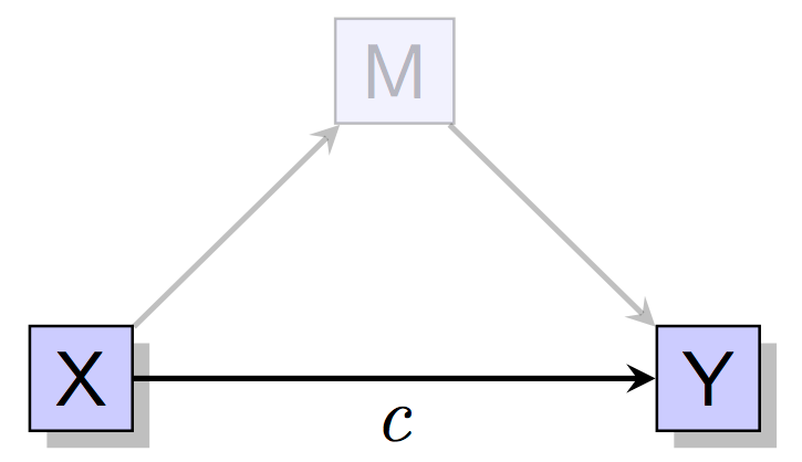
Model 1
First, predict Y from X. Normally one would hope that the relationship \(c\) is significant. However, more modern approaches to mediation analysis do not require that this path is significant. For instance, it could be the case that there are multiple mediating processes, some of which partially cancel each other, and this is why the direct effect is not significant.
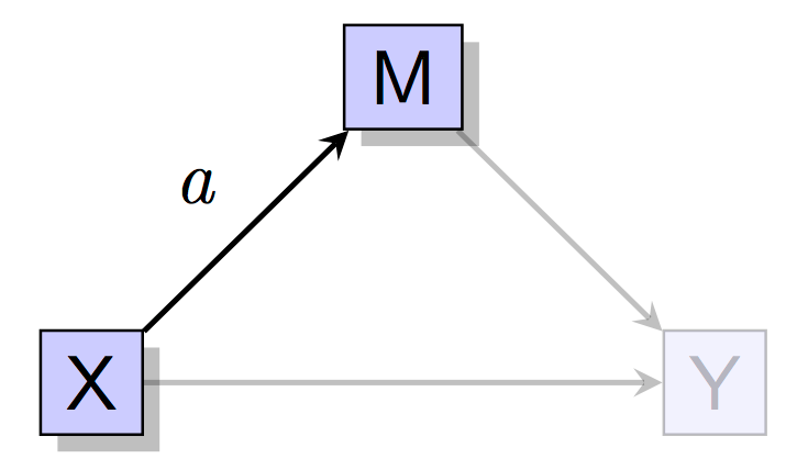
Model 2
Next, predict the M from X and hope that path \(a\) is significant.
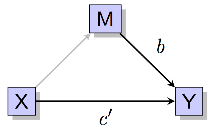
Model 3
Finally, predict the Y from both X and M simultaneously. The coefficient \(b\) tells us whether M predicts Y above and beyond the effect of X. We hope that \(b\) is significant and sometimes it is hoped that \(c'\) is no longer significant, though a lack of a significant relationship here for \(c'\) is not necessarily indicative of complete mediation.
The expected pattern of significance as described above is required for the Baron and Kenny approach to mediation analysis.
Sobel’s test (1982)
Sobel’s test (1982) is a significance test for the indirect effect, \(ab\), and can be used to form a confidence interval. It can be computed from the coefficients for \(a\) and \(b\) and their standard errors. Since it is no longer recommended due to low power, it is not discussed further on this page. If you like you can read Kris Preacher’s page on Soblel’s test here. More modern methods have more power than Sobel’s test and the Baron and Kenny approach (see below), and have shifted towards confidence intervals for the indirect effect rather than just significance testing.
Modern approaches to mediation analysis
Joint signifiance test
The simplest modern variation of the causal steps approach of Baron and Kenny is to simply test the significance of \(a\) and \(b\) coefficients. If both are significant, conclude that there is evidence consistent with an indirect effect. This approach performs well, however, does not yield a single \(p\)-value as does Sobel’s test nor does it yield a confidence interval for the indirect effect.
Partial posterior
The partial posterior approach (Biesanz, Falk, & Savalei, 2010) provides a \(p\)-value for the indirect effect, \(ab\), interpretable in the same way as the \(p\)-value from Sobel’s test. This method has its roots in the statistics literature (Bayarri & Berger, 1999, 2000) in the context of how to make inferences when a sampling distribution depends on a nuisance parameter. This method has higher power than Sobel’s test, power that is comparable to or slightly higher than other modern methods discussed below (e.g., percentile bootstrap and Monte Carlo method), and in most cases appears to adequately control Type I error rates. A version of this approach was also recently studied in the context of structural equation modeling (Falk & Biesanz, 2015). I provide an easy-to-use calculator for the partial posterior method here.
Bootstrapping
Bootstrapping is a resampling method that can be used to construct a confidence interval for the indirect effect, \(ab\). Recent SPSS and SAS macros make use of nonparametric bootstrapping (e.g., Preacher & Hayes, 2004), which can also be accomplished using R, or directly in software such as Mplus and the R package lavaan. Although the percentile bootstrap method performs well in terms of Type I error and power, the bias corrected (BC) and bias corrected and accelerated bootstrap (BCa) methods are not recommended. The BC and BCa approaches tend to have high Type I error rates under some conditions, and 95% confidence intervals are not well calibrated (meaning that they may contain the true indirect effect much less than 95% of the time). Choice of the BC/BCa based on high power may be somewhat misguided (e.g., Biesanz, Falk, & Savalei, 2010; Falk & Biesanz, 2015; Valente et al., 2015).
One downside to bootstrapping is that it requires access to the raw data. In addition, if there is missing data, macros that do bootstrapping will not always appropriately handle missing data (see my FAQ). The analysis performed with each resample must use an appropriate missing data technique (e.g., multiple imputation).
Distribution of the product
The distribution of the product method (MacKinnon et al., 2007) also can be used to create confidence intervals for \(ab\), and maintains good Type I error and power rates. The method relies on an analytical approximation to the distribution of the product of two normally distributed variables. That is, assume that \(a\) and \(b\) have normal sampling distributions, and we want to form a confidence interval based on the product of those sampling distributions. R packages such as RMediation now allow estimation of the distribution of the product.
Monte Carlo method
In its simplest form, the Monte Carlo method may be considered an empirical approximation to the distribution of the product approach. If we consider just a product of coefficients and we assume that the coefficients have a normal sampling distribution (which is reasonable if our sample size is large enough), we can take a large number of random draws from each sampling distribution and multiply the resulting draws together. We can then form a 95% confidence interval by considering the lower/upper 2.5% of the resulting product of coefficients distribution.
The Monte Carlo method is currently more flexible than the distribution of the product approach as it has the potential to more easily form confidence intervals for more complex models (e.g., product of more than 2 coefficients, difference of two coefficients, nonlinear models, etc.). For the simple case of the product of two coefficients, I provide a calculator for the Monte Carlo method. This approach is also available in RMediation and may be used by the mediation package in R. See also calculators on Kris Preacher’s website and Davood Tofighi’s website.
Hierarchical Bayesian method
One Bayesian approach to confidence interval (or credibility interval) estimation is similar to the Monte Carlo method, but takes draws from the posterior distribution of each regression coefficient instead of assuming that the sampling distributions are normal. This approach may be better suited for small samples. This approach was studied by Biesanz et al (2010) and was one of the best performing methods for forming an accurate confidence interval; and for the product of two coefficients, I provide a calculator for the Hierarchical Bayesian method here.
Likelihood-based confidence intervals
Confidence intervals for arbitrary functions of model parameters (such as the product of two coefficients, or the indirect effect) can also be formed by inverting the likelihood-ratio test often used when comparing two alternative models. Such intervals are often asymmetric (around the point estimate for the indirect effect) and called likelihood-based confidence intervals. Such intervals ought to offer similar flexibility to the Monte Carlo method in terms of the complexity of the hypotheses that may be examined; conclusions reached from likelihood-based confidence intervals are also invariant to different parameterizations of the same model (which is not necessarily true of the Monte Carlo approach). Programs such as OpenMx can compute likelihood-based confidence intervals. Falk & Biesanz (2015) studied this approach in the context of a latent variable mediation model and found that it had a slight edge over the percentile bootstrap and distribution of the product methods in terms of power, while maintaining decent Type I error and 95% CI coverage rates. Pek & Wu provide supplementary code for computing such confidence intervals using newer algorithms.
Sensitivity analysis
Sensitivity analysis is not so much a particular method for testing the signifiance of the indirect effect or for forming a confidence interval, but is more an approach of testing the assumptions required for a causal interpretation of the indirect effect. One conceptual way of explaining sensitivity analysis is as follows: Suppose that there are relevant pre-treatment covariates or confounding variables that the researcher fails to measure. A sensitivity analysis may ask how large of an effect such confounding variables must have before our indirect effect disappears. It is important for researchers to consider the assumptions underyling the statements regarding causality that are made when conducting mediation analysis, yet historically this has rarely been done. As of this writing, R packages such as mediation are able to conduct a sensitivity analysis. Methodology researchers have yet to fully integrate the above approaches to interval/inference with that of sensitivity analysis. See also Imai et al. (2010) and the subsection on David Kenny’s page on Causal Inference Approach to Mediation.