Motivation
This post assumes you are interested in doing network modeling and have missing data. To be more specific, suppose you assume that the variables are continuous (or you would like to treat them as such) and you are interested in partial correlations among all variables (the Gaussian graphical model). Quite often we want a network that is parsimonious (i.e., some edges or partial correlations are zero). While the methodology is quickly advancing, one way to do this is to follow this tutorial by Epskamp & Fried (2018), using a lasso that shrinks partial correlations, leading some to become zero, sometimes called the graphical lasso or glasso. The amount of shrinkage is controlled by a tuning parameter that is selected based trying several values and picking the one that minimizes EBIC. All of this can be done easily with a single line of code in an R package such as bootnet (i.e., estimateNetwork with default = "EBICglasso").
But, what happens if there is a sizable amount of missing data? 🤔
This brief tutorial provides some code examples based on recent work by Falk & Starr.1 A few highlights from this paper:
- If doing regularization, “full-information maximum likelihood” in bootnet is not actually FIML; it resembles a two-stage approach from the structural equation modeling (SEM) literature.
- We connect the two-stage approach to the SEM literature to better provide some theoretical justification for it.
- An arguably better approach is to use an EM algorithm, which results in FIML estimates.
- The tuning parameter for the EM algorithm can be chosen in multiple ways; we found that k-fold cross-validation worked slightly better than minimizing EBIC.
Using the EM algorithm with cross-validation (EM-CV) is not difficult. The original development for this approach is from Städler and Bühlmann (2012). I demonstrate it with the EMgaussian R package. Some elements of this tutorial as similar to those in the supplementary materials for Falk & Starr.
Illustration with EM-CV
Setup
First, load necessary packages; an example dataset is from the psych package. We use 25 items, and it has a small amount of missing data. Note in all examples we standardized available values in the raw dataset.
library(EMgaussian)
library(psych)
library(bootnet)
library(qgraph)
library(visdat)
library(lavaan)
For fun, and since bfi does not have a ton of missing data, I decided to induce more missingness. Normally you would not want to do this part. 🙃
data(bfi)

set.seed(1234)
bfi.items <- as.matrix(bfi[,1:25])

bfi.items[sample(1:length(bfi.items), 10000)] <- NA
bfi.items <- as.data.frame(bfi.items)
Initial checks
It’s probably a good idea you look at the missing data patterns, perhaps try to understand the nature of the missingness. This is outside the scope of the current tutorial, but Craig Enders has a nice book. It’s ok if the missigness is missing completely at random (MCAR) or missing at random (MAR), but would not be good for anything that follows if the missingness is missing not at random (MNAR). Sometimes looking at missing data patterns gives clues, sometimes not. Above I induced some MCAR missingness.
Here is one way to look at the missingness:
vis_miss(bfi.items, cluster=TRUE)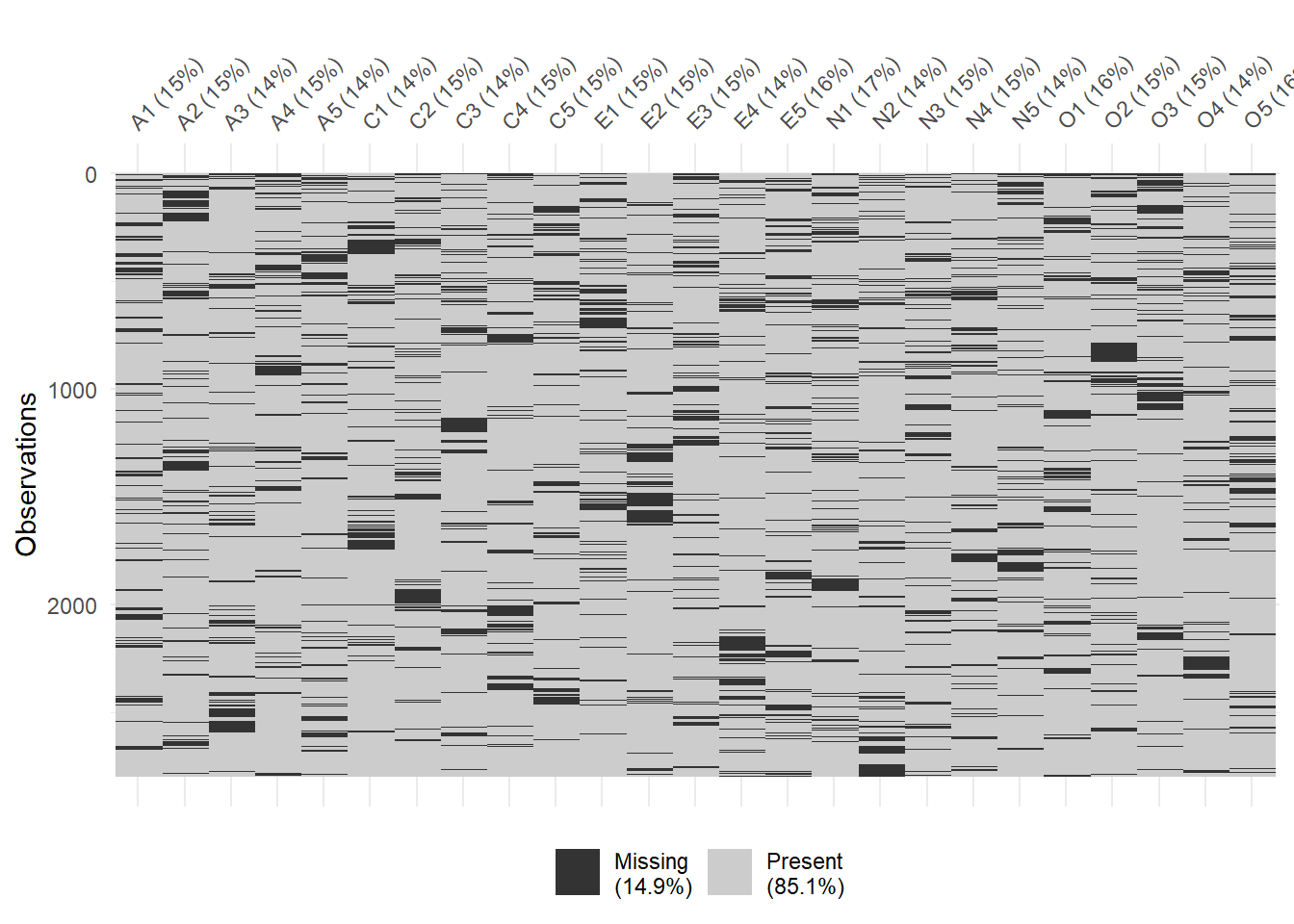
The columns list each variable and the percentage missing. The rows are rows of the dataset, of which there are a lot so they look like tiny slivers. Each row has entries that are either observed (gray) or missing (black). The patterns here look completely random, but sometimes you might notice something interesting - like particular variables that have a lot of missingness (e.g., a question that is sensitive) or once a person has missingness, they stop responding to the remainder of the questions (attrition; assuming the variables are in order of appearance).
It’s also a good idea to check that all variables are observed at least once with every other variable (sometimes called pairwise coverage). That is, it would be a problem if two variables were never observed together at the same time. This is one way to do it, though I’m sure there are better ways:
N <- nrow(bfi.items)
coverage <- lavaan:::lav_data_missing_patterns(bfi.items, coverage=TRUE)$coverage
coverage*N # number of pairwise observations
## A1 A2 A3 A4 A5 C1 C2 C3 C4 C5 E1 E2 E3 E4 E5
## A1 2380 2012 2036 2022 2048 2024 2024 2033 2023 2036 2008 2038 2017 2048 2003
## A2 2012 2380 2048 2036 2062 2036 2029 2032 2034 2039 2017 2031 2018 2032 1999
## A3 2036 2048 2403 2037 2066 2058 2037 2071 2045 2060 2035 2053 2047 2077 2040
## A4 2022 2036 2037 2380 2055 2033 2032 2030 2022 2046 2018 2037 2026 2047 2016
## A5 2048 2062 2066 2055 2412 2069 2054 2048 2048 2074 2049 2064 2056 2074 2030
## C1 2024 2036 2058 2033 2069 2394 2042 2055 2027 2051 2028 2046 2034 2052 2022
## C2 2024 2029 2037 2032 2054 2042 2384 2031 2025 2041 2020 2041 2026 2045 2011
## C3 2033 2032 2071 2030 2048 2055 2031 2397 2051 2042 2038 2045 2036 2051 2026
## C4 2023 2034 2045 2022 2048 2027 2025 2051 2380 2035 2020 2023 2027 2045 2011
## C5 2036 2039 2060 2046 2074 2051 2041 2042 2035 2391 2014 2053 2026 2065 2020
## E1 2008 2017 2035 2018 2049 2028 2020 2038 2020 2014 2371 2027 2009 2028 2009
## E2 2038 2031 2053 2037 2064 2046 2041 2045 2023 2053 2027 2392 2021 2045 2008
## E3 2017 2018 2047 2026 2056 2034 2026 2036 2027 2026 2009 2021 2373 2026 1993
## E4 2048 2032 2077 2047 2074 2052 2045 2051 2045 2065 2028 2045 2026 2400 2020
## E5 2003 1999 2040 2016 2030 2022 2011 2026 2011 2020 2009 2008 1993 2020 2364
## N1 1973 1993 2016 1998 2022 1993 1991 2004 1998 1999 1983 1997 1979 2005 1984
## N2 2040 2040 2055 2031 2063 2050 2027 2053 2041 2036 2020 2044 2025 2055 2012
## N3 2015 2014 2042 2026 2060 2030 2025 2026 2025 2035 2015 2035 2015 2034 2007
## N4 2029 2027 2036 2026 2046 2032 2028 2052 2021 2037 2026 2025 2011 2027 2012
## N5 2052 2059 2068 2056 2073 2060 2056 2069 2057 2053 2049 2067 2043 2068 2044
## O1 1991 2005 2009 1998 2019 1990 2006 2019 1996 2006 1985 2002 1989 2011 1977
## O2 2026 2026 2045 2040 2054 2039 2032 2028 2027 2044 2015 2033 2024 2041 2011
## O3 2016 2017 2044 2024 2039 2027 2013 2044 2010 2033 2009 2015 2002 2029 2012
## O4 2053 2051 2073 2059 2086 2056 2040 2057 2052 2061 2042 2057 2050 2083 2033
## O5 2011 2003 2023 2023 2039 2008 2011 2030 2009 2012 1998 2028 2011 2024 1994
## N1 N2 N3 N4 N5 O1 O2 O3 O4 O5
## A1 1973 2040 2015 2029 2052 1991 2026 2016 2053 2011
## A2 1993 2040 2014 2027 2059 2005 2026 2017 2051 2003
## A3 2016 2055 2042 2036 2068 2009 2045 2044 2073 2023
## A4 1998 2031 2026 2026 2056 1998 2040 2024 2059 2023
## A5 2022 2063 2060 2046 2073 2019 2054 2039 2086 2039
## C1 1993 2050 2030 2032 2060 1990 2039 2027 2056 2008
## C2 1991 2027 2025 2028 2056 2006 2032 2013 2040 2011
## C3 2004 2053 2026 2052 2069 2019 2028 2044 2057 2030
## C4 1998 2041 2025 2021 2057 1996 2027 2010 2052 2009
## C5 1999 2036 2035 2037 2053 2006 2044 2033 2061 2012
## E1 1983 2020 2015 2026 2049 1985 2015 2009 2042 1998
## E2 1997 2044 2035 2025 2067 2002 2033 2015 2057 2028
## E3 1979 2025 2015 2011 2043 1989 2024 2002 2050 2011
## E4 2005 2055 2034 2027 2068 2011 2041 2029 2083 2024
## E5 1984 2012 2007 2012 2044 1977 2011 2012 2033 1994
## N1 2336 1980 1986 1989 2017 1962 1991 1967 2003 1982
## N2 1980 2395 2045 2037 2061 1997 2036 2033 2058 2017
## N3 1986 2045 2377 2023 2048 1989 2031 2022 2052 2003
## N4 1989 2037 2023 2376 2044 1991 2026 2005 2037 2005
## N5 2017 2061 2048 2044 2411 2031 2052 2044 2078 2051
## O1 1962 1997 1989 1991 2031 2348 2010 1990 2024 1996
## O2 1991 2036 2031 2026 2052 2010 2383 2014 2051 2015
## O3 1967 2033 2022 2005 2044 1990 2014 2370 2032 2000
## O4 2003 2058 2052 2037 2078 2024 2051 2032 2410 2030
## O5 1982 2017 2003 2005 2051 1996 2015 2000 2030 2362# are any cases with zero pairwise coverage?
any(coverage*N < 1)## [1] FALSEThe first bit of code computes the number of observations for each variable and pairs of variables, then prints these in a big matrix. For example, there are 2380 observations for variable A1; also, A1 and A2 were observed together 2012 times. It would be a problem if any of the entries here were zero or close to zero. The second bit yields a logical statement regarding whether any cases have zero pairwise coverage. If the logical statement returned TRUE or if some variables were very rarely observed together at the same time, it could be problematic moving forward. Here, we are ok.
Estimation with EM-CV
A grid of candidate tuning parameter values are initially obtained. Here, we obtain 100 possible values. The method used is essentially the same as that used by qgraph but requires an estimate of the covariance matrix; here, we supply the raw data with dat = scale(bfi.items).
rho <- rhogrid(100, method="qgraph", dat = scale(bfi.items))Recall that the tuning parameter controls the amount of penalization, or shrinkage of the partial correlations. Larger tuning parameters will mean more shrinkage of partial correlations.
Next, the EMggm is a custom function provided by EMgaussian that can estimate network models using the EM algorithm with either EBIC or k-fold cross validation to select the “best” tuning parameter. This function currently works in place of some custom function for use with estimateNetwork from the bootnet package.2 Below we use the EM algorithm coupled with cross-validation (EM-CV) with 5 folds to select the tuning parameter.
kfold <- estimateNetwork(scale(bfi.items), fun = EMggm, rho=rho,
                         glassoversion = "glasso", rhoselect = "kfold",
                         k=5)
To be very specific:
scale(bfi.items)is the dataset, standardizedfun = EMggmprovides the custom estimation function from EMgaussianrho = rhopasses the vector of candidate tuning parameter values along, which eventually makes its way toEMggm- This approach was chosen because you might want a different method of candidate tuning parameter values and
rhogridcan do this or you could choose the exact values yourself
- This approach was chosen because you might want a different method of candidate tuning parameter values and
glassoversion = "glasso"determines which R package will do estimation at the M-step of the EM algorithm; the glasso package in R is a typical choice. glassoFast is also possible.rhoselect = "kfold"determines how the “best” value of the tuning parameter is chosen. Here, this corresponds to k-fold cross-validation.k=5is the number of folds (number pieces the dataset is broken up into for the purposes of cross-validation)
The results now stored in kfold can be used as you would results from any undirected network estimated from estimateNetwork. For example, we can obtain plots and centrality indices:
plot(kfold)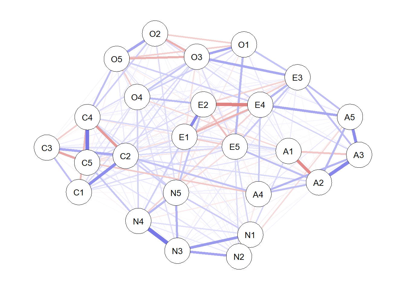
centralityPlot(kfold)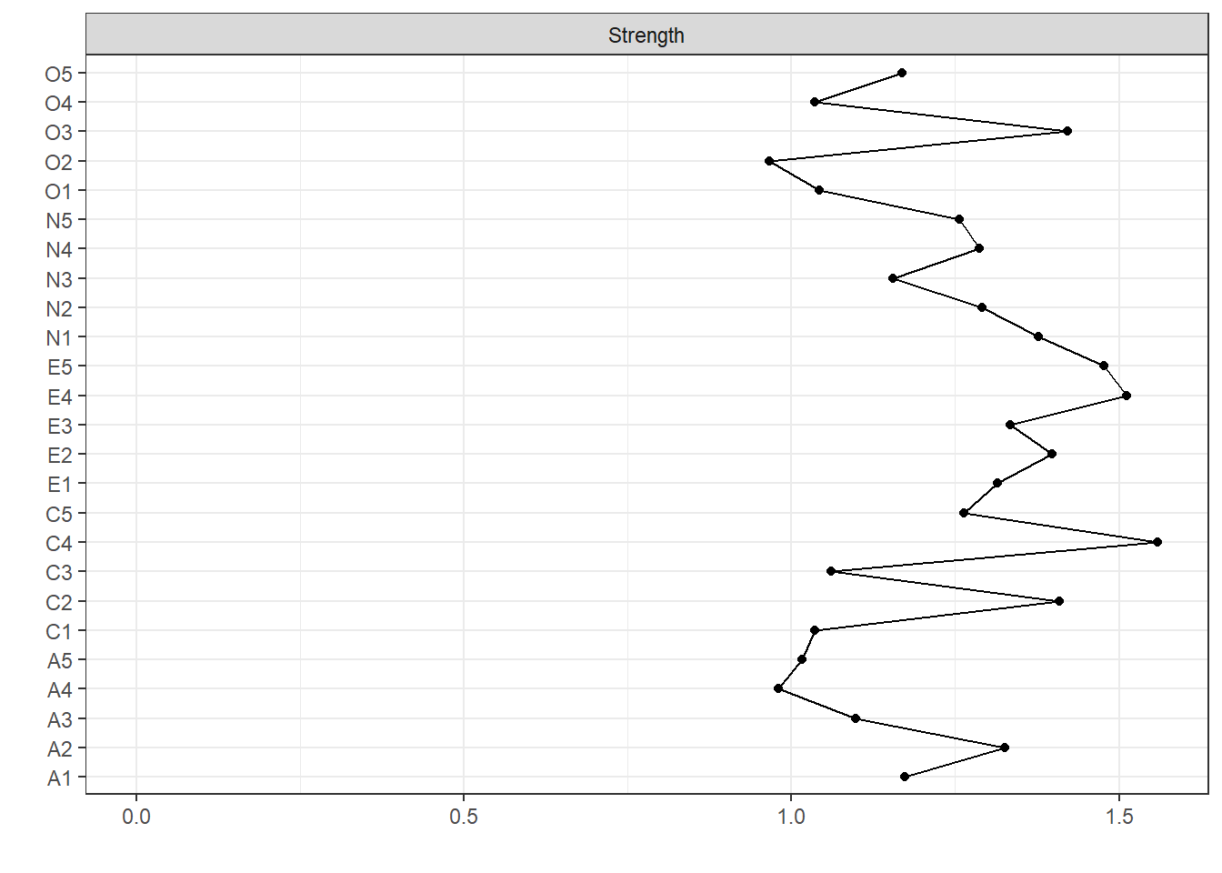
If we want, we could also do bootstrapping to examine network stability as done in the tutorial mentioned at the outset. Though depending on the machine and dataset this can be ridiculously slow.3
#boot1 <- bootnet(kfold, nCores = 15, nBoots = 500, type="nonparametric")
#boot2 <- bootnet(kfold, nCores = 15, nBoots = 500, type="case")
Output, such as the grid of tuning parameter values, criterion (k-fold), are also accessible.
kfold$results$rho # grid of tuning parameter values## [1] 0.007127529 0.007466911 0.007822454 0.008194926 0.008585134 0.008993921
## [7] 0.009422173 0.009870817 0.010340824 0.010833210 0.011349041 0.011889434
## [13] 0.012455559 0.013048640 0.013669960 0.014320866 0.015002765 0.015717133
## [19] 0.016465516 0.017249534 0.018070883 0.018931342 0.019832772 0.020777124
## [25] 0.021766443 0.022802868 0.023888644 0.025026120 0.026217757 0.027466136
## [31] 0.028773956 0.030144050 0.031579382 0.033083058 0.034658332 0.036308615
## [37] 0.038037477 0.039848660 0.041746084 0.043733855 0.045816276 0.047997852
## [43] 0.050283306 0.052677583 0.055185866 0.057813583 0.060566420 0.063450336
## [49] 0.066471571 0.069636665 0.072952467 0.076426154 0.080065243 0.083877610
## [55] 0.087871505 0.092055573 0.096438869 0.101030878 0.105841539 0.110881264
## [61] 0.116160959 0.121692050 0.127486509 0.133556875 0.139916286 0.146578505
## [67] 0.153557951 0.160869729 0.168529662 0.176554328 0.184961096 0.193768158
## [73] 0.202994574 0.212660314 0.222786295 0.233394432 0.244507683 0.256150101
## [79] 0.268346881 0.281124419 0.294510370 0.308533703 0.323224768 0.338615358
## [85] 0.354738783 0.371629938 0.389325377 0.407863398 0.427284121 0.447629576
## [91] 0.468943795 0.491272907 0.514665236 0.539171409 0.564844461 0.591739955
## [97] 0.619916099 0.649433870 0.680357153 0.712752871kfold$results$crit # criterion (EBIC or cross-validation) @ each tuning parameter## [1] 86715.24 86717.16 86719.39 86722.03 86725.01 86728.33 86731.86 86735.71
## [9] 86739.97 86744.66 86749.80 86755.30 86761.17 86767.41 86774.30 86781.83
## [17] 86790.21 86799.51 86809.55 86820.43 86832.20 86844.88 86858.37 86872.93
## [25] 86888.65 86905.68 86924.20 86944.37 86966.22 86989.55 87014.28 87040.42
## [33] 87068.12 87097.33 87128.30 87161.51 87197.15 87234.52 87274.02 87315.91
## [41] 87359.98 87406.20 87455.24 87507.67 87563.76 87623.47 87686.07 87752.18
## [49] 87822.72 87898.03 87976.70 88059.37 88147.08 88240.93 88342.01 88451.32
## [57] 88569.55 88697.35 88835.56 88984.46 89144.95 89317.94 89503.57 89701.51
## [65] 89909.98 90130.06 90366.21 90618.16 90883.83 91160.49 91449.76 91749.80
## [73] 92062.25 92382.06 92706.58 93033.18 93364.93 93698.50 94018.45 94311.15
## [81] 94584.61 94833.12 95059.10 95278.33 95487.21 95684.59 95873.38 96052.28
## [89] 96220.42 96396.77 96582.91 96779.25 96981.85 97185.47 97399.44 97625.76
## [97] 97864.87 98117.24 98383.31 98663.54kfold$results$it # number of EM cycles performed## [1] 16kfold$results$conv # convergence code## [1] TRUEIf you wanted to know which value of the tuning parameter was chosen…
kfold$results$rho[which.min(kfold$results$crit)]## [1] 0.007127529Other estimation options
EM algorithm with EBIC to select the tuning parameter
Although not the best approach in Falk & Starr’s paper, the EM algorithm could also be coupled with minimizing EBIC to select the tuning parameter. This approach arguably did better than the two-stage approach that’s built into bootnet An example is as follows, which is the same as code for EM-CV, except rhoselect = "ebic" and there is no need to specify the number of folds.
ebic <- estimateNetwork(scale(bfi.items), fun = EMggm, rho=rho,
                         glassoversion = "glasso", rhoselect = "ebic")
Not penalizing the diagonal of the precision matrix
Note that the above examples estimate the model while penalizing the diagonal of the precision matrix. In supplementary materials of the manuscript, we note that whether this is done does not appear to have an impact on the relative performance of the methods. However, not penalizing the diagonal of the precision matrix is also easily possible, and may result in fewer null matrices with EM-EBIC, but sometimes slightly worse recovery of partial correlations or node strength, particularly at the smallest sample sizes. The following example code does not penalize the diagonal and is illustrated for EM-EBIC and EM-CV:
ebic <- estimateNetwork(scale(bfi.items), fun = EMggm, rho=rho,
                         glassoversion = "glasso", rhoselect = "ebic",
                         penalize.diagonal = FALSE)

kfold <- estimateNetwork(scale(bfi.items), fun = EMggm, rho=rho,
                         glassoversion = "glasso", rhoselect = "kfold",
                         k=5, penalize.diagonal = FALSE)
Here, we just added penalize.diagonal = FALSE, which is an option available if glassoversion = "glasso".
Two-stage approach from bootnet
The two-stage approach studied in the paper resembles the following:
# EBIC with bootnet; two-stage estimation
ebic.ts <- estimateNetwork(scale(bfi.items), default="EBICglasso",
                           corMethod="cor_auto",
                           sampleSize = "pairwise_average",
                           missing="fiml")
## Estimating Network. Using package::function:
## - qgraph::EBICglasso for EBIC model selection
## - using glasso::glasso
## - qgraph::cor_auto for correlation computation
## - using lavaan::lavCor## Warning in EBICglassoCore(S = S, n = n, gamma = gamma, penalize.diagonal =
## penalize.diagonal, : A dense regularized network was selected (lambda < 0.1 *
## lambda.max). Recent work indicates a possible drop in specificity. Interpret
## the presence of the smallest edges with care. Setting threshold = TRUE will
## enforce higher specificity, at the cost of sensitivity.Note that even though the code says missing="fiml", this approach is not quite FIML in the truest sense. The covariance matrix among all variables is first estimated with FIML, actually using lavaan and an EM algorithm under the hood. Then, this covariance matrix is treated as “known” in a second stage where regularization is done, the tuning parameter is selected, and we end up with a final estimate of the precision matrix. This approach has been available in bootnet for a long time, but to my knowledge not clearly articulated in the literature.
This two-stage approach is not quite as good as using EM-CV or EM-EBIC. But, the Falk & Starr paper establishes some theoretical justification for it, in part by making the connection to the SEM literature. Note that Nehler & Schultze (2025) also study the two-stage approach, but make little connection to the SEM literature and do not provide supporting technical details. Their study is in agreement with ours that the two-stage approach is not quite as good as use of the EM algorithm. The history of the two-stage approach in SEM I will not go into, but it initially arose as a way of handling missing data in SEM that was not ideal, but was feasible at the time. In this case, if sample size is large and you used the two-stage approach before, I would not worry too much. If sample size is small and/or there is a ton of missing data, then something else like EM-CV is likely much better.
Conclusion
Estimating regularized network models under missing data should not be that difficult anymore. This post presents a couple of options for the Gaussian graphical model with a lasso. 👍
What to report about estimation?
In addition to anything recommended by other tutorials, like the one mentioned at the outset of this blog post…
- How many tuning parameters you evaluated and the method used to obtain them
- Here, we evaluated 100 tuning parameters. The candidate tuning parameters were determined using the method employed by
qgraph. The details are a bit technical (seehelp(rhogrid)).
- Here, we evaluated 100 tuning parameters. The candidate tuning parameters were determined using the method employed by
- Whether you use the expectation maximization (EM) algorithm with \(k\)-fold cross-validation to select the tuning parameter (with the number of folds; here, 5 folds), or if you use the EM algorithm with EBIC to select the tuning parameter.
- Whether you used glasso or glassoFast
- Whether the diagonal of the precision matrix was penalized (glassoFast always penalizes, with glasso you have a choice)
Citation
I guess if you want to cite this blog post, you could.
Falk, C. F. (2025, August 20). Regularized (lasso) network modeling with high rates of missing data. https://www.psych.mcgill.ca/perpg/fac/falk/post/2025/08/12/regularized-(lasso)-network-modeling-with-high-missing-data/
Though it would probably make more sense to cite the paper that this comes from and the EMgaussian package if you use it.
Falk, C. F., & Starr, J. (in press). Regularized cross-sectional network modeling with missing data: A comparison of methods. Multivariate Behavioral Research.
Falk, C.F. (2025). EMgaussian: Expectation-Maximization Algorithm for Multivariate Normal (Gaussian) with Missing Data. R package version 0.2.2, https://CRAN.R-project.org/package=EMgaussian.
And if you used bootnet and glasso as my code examples do, cite those as well. Examples below, at least at the time of writing.
Epskamp, S., Borsboom, D., & Fried, E. I. (2018). Estimating psychological networks and their accuracy: A tutorial paper. Behavior Research Methods, 50, 195-212.
Friedman J., Hastie T., Tibshirani, R. (2019). glasso: Graphical Lasso: Estimation of Gaussian Graphical Models. R package version 1.11, https://CRAN.R-project.org/package=glasso.
If you are using EM-CV, the original methodological development:
Städler, N., & Bühlmann, P. (2012). Missing values: sparse inverse covariance estimation and an extension to sparse regression. Statistics and Computing, 22, 219–235.
This work has recently been accepted for publication in Multivariate Behavioral Research and is currently in production.↩︎
Thanks to the bootnet developers for making this function flexible enough to use a custom estimation approach!↩︎
EMgaussian would be a bit faster if some code changes under the hood were to take place, such as grouping by missing data pattern. Anyone interested in coding?↩︎