Mediation Analysis
An old tutorial that introduced a few methods that I studied and published on in the early 2010’s. Contains instruction and source code to these programs and may still be useful for doing analyses from published research papers.
Overview
Note: This tutorial was initially published on an older version of my website in approximately 2015, and has only been lightly edited since. The content introducing mediation analysis is in need of updating, and in particular the assumptions and proper specification of mediation analysis models so as to have a better understanding of the involved causal processes, advantages of using longitudinal (instead of cross-sectional) data, and so on.
So, you have been warned. The rest of this post is still here for a couple of reasons: 1) historical purposes as it contains reference to some computer programs/code developed in the context of a few publications; 2) some of the calculators here do not necessarily require access to the raw data, meaning they could be applied to published research articles.
To add to the above, a few articles/chapters that may be of interest. Not comprehensive list since a ton has been written on the topic, and no one quite covers everything.
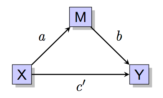
Researchers in psychology and other social sciences are often interested in performing mediation analysis to explain the relationship between an independent variable (X) and dependent variable (Y) in terms of a third hypothesized process or mediating variable (M). Often there is a hypothesis that the variables are causally related. For instance, it is often hypothesized that X causes changes in M, represented by the coefficient \(a\) in the Figure below, and that M causes changes in Y as represented by the coefficient \(b\). Assuming all continuous variables, the product of the coefficients \(ab\) is called the indirect effect of X on Y that passes through M.
Traditional approaches to mediation analysis
Sobel’s test (1982) and the Baron and Kenny approach (1986) are common methods of testing hypotheses regarding mediation analysis. Both methods have low power compared to more modern approaches and are typically no longer recommended (e.g., MacKinnon et al., 2002; Biesanz, Falk, & Savalei, 2010).
Baron & Kenny (1986)
The Baron and Kenny approach consists of fitting 3 different models to the data.
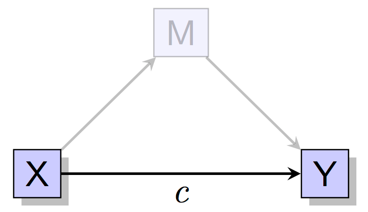
Model 1
First, predict Y from X. Normally one would hope that the relationship \(c\) is significant. However, more modern approaches to mediation analysis do not require that this path is significant. For instance, it could be the case that there are multiple mediating processes, some of which partially cancel each other, and this is why the direct effect is not significant.
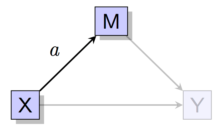
Model 2
Next, predict the M from X and hope that path \(a\) is significant.
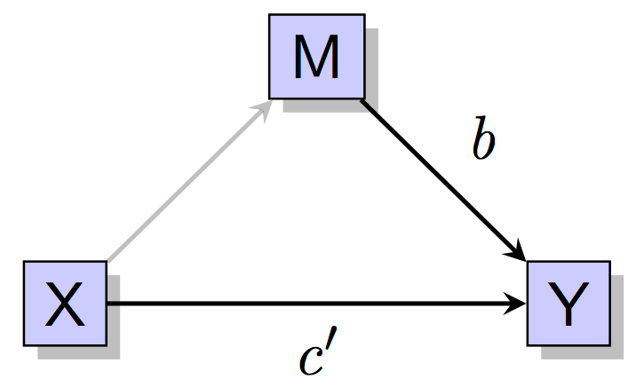
Model 3
Finally, predict the Y from both X and M simultaneously. The coefficient \(b\) tells us whether M predicts Y above and beyond the effect of X. We hope that \(b\) is significant and sometimes it is hoped that \(c'\) is no longer significant, though a lack of a significant relationship here for \(c'\) is not necessarily indicative of complete mediation.
The expected pattern of significance as described above is required for the Baron and Kenny approach to mediation analysis.
Sobel’s test (1982)
Sobel’s test (1982) is a significance test for the indirect effect, \(ab\), and can be used to form a confidence interval. It can be computed from the coefficients for \(a\) and \(b\) and their standard errors. Since it is no longer recommended due to low power, it is not discussed further on this page. If you like you can read Kris Preacher’s page on Sobel’s test here. More modern methods have more power than Sobel’s test and the Baron and Kenny approach (see below), and have shifted towards confidence intervals for the indirect effect rather than just significance testing.
Modern approaches to mediation analysis
Joint signifiance test
The simplest modern variation of the causal steps approach of Baron and Kenny is to simply test the significance of \(a\) and \(b\) coefficients. If both are significant, conclude that there is evidence consistent with an indirect effect. This approach performs well, however, does not yield a single p-value as does Sobel’s test nor does it yield a confidence interval for the indirect effect.
Partial posterior
The partial posterior approach (Biesanz, Falk, & Savalei, 2010) provides a p-value for the indirect effect, \(ab\), interpretable in the same way as the p-value from Sobel’s test. This method has its roots in the statistics literature (Bayarri & Berger, 1999, 2000) in the context of how to make inferences when a sampling distribution depends on a nuisance parameter. This method has higher power than Sobel’s test, power that is comparable to or slightly higher than other modern methods discussed below (e.g., percentile bootstrap and Monte Carlo method), and in most cases appears to adequately control Type I error rates. A version of this approach was also recently studied in the context of structural equation modeling (Falk & Biesanz, 2015). I provide a calculator for the partial posterior method here.
Bootstrapping
Bootstrapping is a resampling method that can be used to construct a confidence interval for the indirect effect, \(ab\). SPSS and SAS macros make use of nonparametric bootstrapping (e.g., Preacher & Hayes, 2004), which can also be accomplished using R, or directly in software such as Mplus and the R package lavaan. Although the percentile bootstrap method performs well in terms of Type I error and power, the bias corrected (BC) and bias corrected and accelerated bootstrap (BCa) methods are not recommended. The BC and BCa approaches tend to have high Type I error rates under some conditions, and 95% confidence intervals are not well calibrated (meaning that they may contain the true indirect effect much less than 95% of the time). Choice of the BC/BCa based on high power may be somewhat misguided (e.g., Biesanz, Falk, & Savalei, 2010; Falk & Biesanz, 2015; Valente et al., 2015).
One downside to bootstrapping is that it requires access to the raw data. In addition, if there is missing data, macros that do bootstrapping will not always appropriately handle missing data (see the FAQ). The analysis performed with each resample must use an appropriate missing data technique (e.g., multiple imputation).
Distribution of the product
The distribution of the product method (MacKinnon et al., 2007) also can be used to create confidence intervals for \(ab\), and maintains good Type I error and power rates. The method relies on an analytical approximation to the distribution of the product of two normally distributed variables. That is, assume that \(a\) and \(b\) have normal sampling distributions, and we want to form a confidence interval based on the product of those sampling distributions. R packages such as RMediation now allow estimation of the distribution of the product.
Monte Carlo method
In its simplest form, the Monte Carlo method may be considered an empirical approximation to the distribution of the product approach. If we consider just a product of coefficients and we assume that the coefficients have a normal sampling distribution (which is reasonable if our sample size is large enough), we can take a large number of random draws from each sampling distribution and multiply the resulting draws together. We can then form a 95% confidence interval by considering the lower/upper 2.5% of the resulting product of coefficients distribution.
The Monte Carlo method is currently more flexible than the distribution of the product approach as it has the potential to more easily form confidence intervals for more complex models (e.g., product of more than 2 coefficients, difference of two coefficients, nonlinear models, etc.). For the simple case of the product of two coefficients, I provide a calculator for the Monte Carlo method. This approach is also available in RMediation and may be used by the mediation package in R. See also calculators on Kris Preacher’s website and Davood Tofighi’s website.
Hierarchical Bayesian method
One Bayesian approach to confidence interval (or credibility interval) estimation is similar to the Monte Carlo method, but takes draws from the posterior distribution of each regression coefficient instead of assuming that the sampling distributions are normal. This approach may be better suited for small samples. This approach was studied by Biesanz et al (2010) and was one of the best performing methods for forming an accurate confidence interval; and for the product of two coefficients, I provide a calculator for the Hierarchical Bayesian method here.
Likelihood-based confidence intervals
Confidence intervals for arbitrary functions of model parameters (such as the product of two coefficients, or the indirect effect) can also be formed by inverting the likelihood-ratio test often used when comparing two alternative models. Such intervals are often asymmetric (around the point estimate for the indirect effect) and called likelihood-based confidence intervals. Such intervals ought to offer similar flexibility to the Monte Carlo method in terms of the complexity of the hypotheses that may be examined; conclusions reached from likelihood-based confidence intervals are also invariant to different parameterizations of the same model (which is not necessarily true of the Monte Carlo approach). OpenMx can compute likelihood-based confidence intervals. Falk & Biesanz (2015) studied this approach in the context of a latent variable mediation model and found that it had a slight edge over the percentile bootstrap and distribution of the product methods in terms of power, while maintaining decent Type I error and 95% CI coverage rates. Pek & Wu provide supplementary code for computing such confidence intervals using newer algorithms.
Sensitivity analysis
Sensitivity analysis is not so much a particular method for testing the significance of the indirect effect or for forming a confidence interval, but is more an approach of testing the assumptions required for a causal interpretation of the indirect effect. One conceptual way of explaining sensitivity analysis is as follows: Suppose that there are relevant pre-treatment covariates or confounding variables that the researcher fails to measure. A sensitivity analysis may ask how large of an effect such confounding variables must have before our indirect effect disappears. It is important for researchers to consider the assumptions underyling the statements regarding causality that are made when conducting mediation analysis, yet historically this has rarely been done. As of this writing, R packages such as mediation are able to conduct a sensitivity analysis. Methodology researchers have yet to fully integrate the above approaches to interval/inference with that of sensitivity analysis. See also Imai et al. (2010) and the subsection on David Kenny’s page on Causal Inference Approach to Mediation.
Calculators for mediation analysis
This section discusses two programs for computing (1) p-values and (2) confidence intervals for the indirect effect. Both programs are intended to be easy-to-use, do not require commercial statistical software, do not require editing of SPSS or SAS syntax, and do not require the raw data. The user only needs to input information that one would normally need to obtain anyway if performing mediation analysis using traditional methods (e.g., regression coefficients, standard errors, degrees of freedom, and t-statistics).
Within each program, there are two computational methods - one method where sampling distributions are based in-part on posterior (and t) distributions (appropriate for regression models), and a second method where normal approximations are used in place of posterior distributions (appropriate for larger samples or methods where such normal approximations are used, such as structural equation models).
p-values are computed by the partial posterior method. In Biesanz et al (2010), the partial posterior approach had high power relative to traditional approaches, power on par with the modern approaches just described, and adequately controlled Type I error rates. Furthermore, the partial posterior provides a single p-value interpretable in the same way as one would interpret the p-value from Sobel’s test. The use of normal approximations in adapting the partial posterior method to structural equation models also performed well at sample sizes above 100 in a recent simulation study (Falk & Biesanz, 2015).
Confidence intervals are available from the hierarchical Bayesian and Monte Carlo methods. In Biesanz et al (2010), the hierarchical Bayesian method provided coverage rates for the indirect effect that outperformed both the distribution of the product method and the BCa bootstrap. The Monte Carlo method performs similarly to the hierarchical Bayesian method and distribution of the product method at large sample sizes. The Monte Carlo method is also appropriate for confidence intervals in structural equation models as it allows for a correlation between the two paths in the model (which is not necessarily 0 in models that contain latent variables).
Indirect effect confidence interval calculator
This page provides a brief tutorial for the confidence interval calculator described in Falk & Biesanz (2016). The program is intended to be easy-to-use, does not require commercial statistical software, does not require editing of SPSS or SAS syntax, and does not require the raw data. The user only needs to input information that one would normally need to obtain anyway if performing mediation analysis using traditional methods (e.g., regression coefficients, standard errors, degrees of freedom, and t-statistics).
Within the program, there are two computational methods - one method where sampling distributions are based in-part on posterior (and t) distributions (appropriate for regression models), and a second method where normal approximations are used in place of posterior distributions (appropriate for larger samples or methods where such normal approximations are used, such as structural equation models).
Confidence intervals are available from the hierarchical Bayesian (appropriate for multiple regression models) and Monte Carlo methods (appropriate for structural equation and some multilevel models - see FAQ on use of some multilevel models). In Biesanz et al (2010), the hierarchical Bayesian method provided coverage rates for the indirect effect that outperformed both the distribution of the product method and the BCa bootstrap. The Monte Carlo method performs similarly to the hierarchical Bayesian method and distribution of the product method at large sample sizes. The Monte Carlo method is also appropriate for confidence intervals in structural equation models as it allows for a correlation between the two paths in the model (which is not necessarily 0 in models that contain latent variables).
Users of the confidence interval calculator calculator may cite:
Falk, C.F., & Biesanz, J.C. (2016). Two cross-platform programs for inferences and interval estimation about indirect effects in mediational models. SAGE Open, 6. https://dx.doi.org/10.1177/2158244015625445
Instructions on program use
Click on the link below to download the program.
MediationCI.jar (last update: 2015-08-18)
Once downloaded, double click on the file and it will open in a new window. For some users, it may require an update/install to a new version of Java Runtime Environment: https://java.com/en/download/.
This program is computationally intensive. So far the program has been tested under Windows XP, Windows 7, and OSX (Mac) version 10.7.3 (Lion). If you encounter any problems with the program, please report them directly to me: carl.falk@mcgill.ca
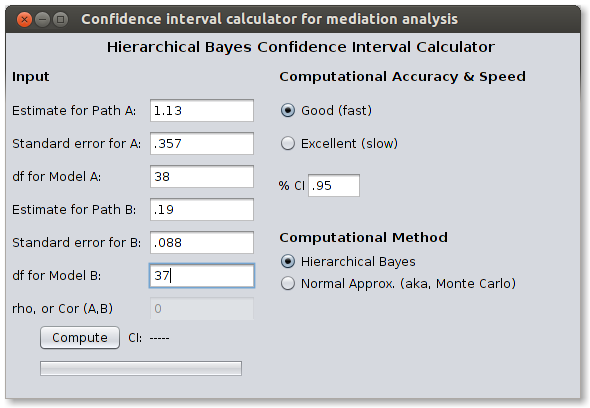
After the program loads, the next step is to enter the regression coefficient, standard error, and degrees of freedom for the a path in the mediational model. In the empirical example in Biesanz, Falk, and Savalei (2010), these values are 1.13, .357, and 38, respectively. After that, enter the regression coefficient, standard errors, and degress of freedom for the b path in the mediation model. In the empirical example in Biesanz, Falk, and Savalei (2010), these values are .19, .088, and 37. The result of these two steps is shown below. If the paths are part of a structural equation model, omit the df, select “Normal approx.” as the computational method, and enter the correlation between the two paths of the model (obtained from the variance-covariance matrix of model parameters).
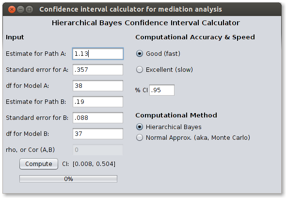
Next click “Compute” and the program will get to work. Note that “Good” computational accuracy will usually take just a couple minutes and is recommended for general use. Researchers wishing a higher level of stability (e.g., confidence intervals that vary less from run to run) for publication may use the “Excellent” computational accuracy setting, but must be prepared to be very patient.
The result of the program is now displayed below. The confidence interval does not contain zero, but includes values from .008 to .504.
Source code
Source code for the confidence interval calculator is available here and is distributable/modifiable under the GPL-3:
This program makes use of the Stochastic Simulation in Java libraries (open source statistical libraries) Java available here.
Indirect effect p-value calculator
This section provides a brief tutorial for the p-value calculator described in Falk & Biesanz (2016). The program is intended to be easy-to-use, does not require commercial statistical software, does not require editing of SPSS or SAS syntax, and does not require the raw data.The user only needs to input information that one would normally need to obtain anyway if performing mediation analysis using traditional methods (e.g., regression coefficients, standard errors, degrees of freedom, and t-statistics).
Within the program, there are two computational methods - one method where sampling distributions are based in-part on posterior (and t) distributions (appropriate for regression models), and a second method where normal approximations are used in place of posterior distributions (appropriate for larger samples or methods where such normal approximations are used, such as structural equation models).
P-values are computed by the partial posterior method - a high-power alternative to Sobel’s test. In Biesanz et al (2010), the partial posterior approach had high power relative to traditional approaches, power on par with the modern approaches just described, and adequately controlled Type I error rates. The calculator may be used for making inferences about indirect effects with multiple regression models (t-distribution computational method), or structural equation or certain multilevel models (see also FAQ about multilevel models) when degree of freedom approximations are not available (normal approximation). Furthermore, the partial posterior provides a single p-value interpretable in the same way as one would interpret the p-value from Sobel’s test. The use of normal approximations in adapting the partial posterior method to structural equation models also performed well at sample sizes above 100 in a recent simulation study (Falk & Biesanz, 2015).
Users of the p-value calculator calculator may cite:
Falk, C.F., & Biesanz, J.C. (2016). Two cross-platform programs for inferences and interval estimation about indirect effects in mediational models. SAGE Open, 6. https://dx.doi.org/10.1177/2158244015625445
Instructions on program use
Click on the link below to download the program.
MediationPval.jar (last update: 2015-08-18)
Once downloaded, double click on the file and it will open in a new window. For some users, it may require an update/install to a new version of Java Runtime Environment: https://java.com/en/download/.
This program is computationally intensive. The program has been tested under Windows XP, Windows 7, and OSX (Mac) version 10.7.3 (Lion). If you encounter any problems with the program, please report them directly to me: carl.falk@mcgill.ca
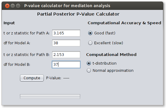
After the program loads, the next step is to enter the t-statistic and degrees of freedom for the a path in the mediation model. In the empirical example in Biesanz, Falk, and Savalei (2010), the t-statistic is 3.165 with df of 38. After that, enter the t-statistic and degrees of freedom for the b path in the mediational model. In the empirical example in Biesanz, Falk, and Savalei (2010), the t-statistic is 2.153 with df of 37. The result of these two steps is shown below. If the paths are part of a structural equation model, enter the z-statistics for the two paths, and select “Normal approximation” as the computational method (no df necessary).
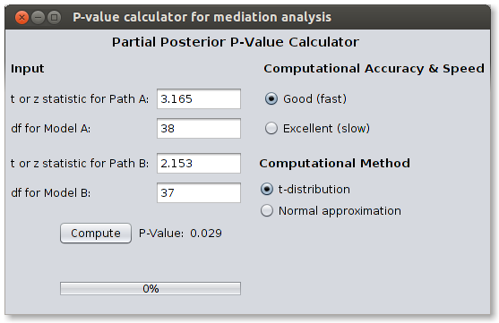
Next click “Compute” and the program will get to work. Note that “Good” computational accuracy will usually take just a couple minutes and is recommended for general use. Researchers wishing a higher level of stability (e.g., p-values that vary less from run to run) for publication may use the “Excellent” computational accuracy setting, but must be prepared to be very patient.
The result of the program is now displayed below (.029), which is significant at the alpha = .05 level. Thus, the indirect effect, ab is significant in this example. Evidence consistent with mediation has been found.
Source code
Source code for the p-value calculator is available here and is distributable/modifiable under the GPL-3:
This program makes use of the Stochastic Simulation in Java libraries (open source statistical libraries) available here
R code
R code and data for the empirical example in Biesanz, Falk, and Savalei (2010), can be found below. This code demonstrates all methods with complete data, missing data, and includes the partial posterior method.
Additional References
An example for writing up the results from a mediation analysis that uses the partial posterior method may be found in the following paper (end of p. 26): Human, Biesanz, Parisotto, and Dunn (2012), or in Falk & Biesanz (2016). The method using t-statistics was presented and studied by Biesanz et al. (2010), and the method using the normal approximation with structural equation models was initially studied by Falk & Biesanz (2015).
Human, L.J., Biesanz, J.C., Parisotto, K.L., & Dunn, E.W. (2012). Your best self helps reveal your true self: Positive self-presentation leads to more accurate personality impressions. Social Psychological and Personality Science, 3, 23-30. https://dx.doi.org/10.1177/1948550611407689
Biesanz, J.C., Falk, C.F., & Savalei, V. (2010). Assessing mediational models: Testing and interval estimation for indirect effects. Multivariate Behavioral Research, 45, 661-701. https://dx.doi.org/10.1080/00273171.2010.498292
Falk, C.F., & Biesanz, J.C. (2015). Inference and interval estimation methods for indirect effects with latent variable models. Structural Equation Modeling, 22, 24-38. https://dx.doi.org/10.1080/10705511.2014.935266
FAQ and Links
- Can the calculators on this page be used to analyze mediation analysis results from published research?
In principle the calculators can be used for this purpose. One motivation behind implementing these particular methods is that only summary information from an analysis is required in order to compute inference and intervals for the indirect effect. The raw data is not required as it is for resampling methods such as bootstrapping. If there is missing data or non-normality, it is desirable that the original analyst has chosen an appropriate modeling technique to account for this. In addition, one is not tied to a particular proprietary statistical package in order to use these calculators; you may use whatever statistical program you choose to estimate the appropriate regression models, structural equation models, or hierarchical linear models.
- Can the calculators on this page be used if there is missing data in my dataset?
Yes, provided that the missingness is appropriately handled through a technique such as multiple imputation, or so-called full information maximum likelihood (using the term in the structural equation modeling literature). If this is done, then you can just use the point estimates and standard errors from such an analysis and use directly in the above calculators. Biesanz et al (2010) conducted simulations using the partial posterior and Hierarchical Bayesian approaches with similar techniques, and R code is also provided below. If you have a substantial amount of missing data, be wary of approaches that use so-called listwise deletion as this is not an ideal approach. For instance, at the time this page was initially written (and still true as I skim this in 2026), Andrew Hayes’ PROCESS macro for SPSS and SAS can apparently only handle complete data and will do listwise deletion by default, e.g., see the FAQ for PROCESS.
- Can the calculators on this page be used with nonlinear models (e.g., dichotomous mediator and outcome)?
No. They were not designed for such use. The R package mediation may also be of help, as is Mplus code that used to be linked to on Andrew Hayes’ website (maybe it moved).
- Can the calculators on this page do sensitivity analysis?
No. The best resource I am aware of at this time is the mediation R package.
- Can I use these calculators with multilevel models?
It depends a little on the design and at what level are the measured predictor, mediator, and outcome. If 2-2-1 or 2-1-1, then the calculators may be ok options. If mediation is all at level 1, then usually I would start with reading this paper: Bauer, Preacher, Gil (2006), and look here if your slopes are all random: https://quantpsy.org/medmc/medmc111.htm Kris Preacher’s website. I created the R package multilevelmediation to handle this case, and it accompanies Falk et al (2024). A possible critique is that this still handles just this classic model and many more advanced approaches have been developed since. For example, centering could be done better and see this note from Dan Bauer regarding this. And there are also longitudinal models in the the structural equation modeling framework that could be used.
Below are some additional links to other pages with information, tutorials, programs, etc. about mediation analysis and indirect effects (deadlinks removed in 2026).
- David Kenny’s page on mediation analysis
- Kristopher Preacher’s page on mediation and moderation
- Sobel Test Calculator (not recommended due to low power and poor CI coverage rates)
- mediation (R package that includes sensitivity analysis)
- RMediation (R package that will do distribution of the product and Monte Carlo method)
- Davood Tofighi’s website (has version of app that will do product of more than 2 coefficients)
- Examples of Mplus code for mediation and moderation by Chris Stride