Profile Estimation Experiments - the Rossler Equations
This page provides code to run profiled parameter estimation on data generated by the Rossler equations. It follows the same format as FhNEx.html and has commentary has therefore been kept to a minimum.
The Rossler equations are given by


Contents
- Path Functions
- Various parameters
- Observation times
- Create paths
- Set up observations
- Fitting parameters
- Profiling optimisation control
- Setting up functional data objects
- Smooth the data
- Re-smoothing with model-based penalty
- Perform the Profiled Estimation
- Plot Smooth with Profile-Estimated Parameters
- Comparison with Smooth Using True Parameters
- Squared Error Performance
- Calculate Sample Information and Variance-Covariance Matrices
Path Functions
odefn    = @rossfun1;      % Function for ODE solver

fn       = @rossfun;       % RHS function
dfdy     = @rossdfdy;      % Derivative wrt inputs
dfdp     = @rossdfdp;      % Derviative wrt parameters

d2fdy2   = @rossd2fdy2;    % Hessian wrt inputs
d2fdydp  = @rossd2fdydp;   % Hessian wrt inputs and parameters
d2fdp2   = @rossd2fdp2;    % Hessian wrt parameters.

d3fdy3   = @rossd3fdy3;    % Third derivative wrt inputs.
d3fdy2dp = @rossd3fdy2dp;  % Third derivative wrt intputs, inputs and pars.
d3fdydp2 = @rossd3fdydp2;  % Third derivative wrt inputs, pars and pars.
Various parameters
y0 = [1.13293; -1.74953; 0.02207];       % Initial conditions

pars = [0.2; 0.2; 3];           % Parameters

sigma = 0.5;                    % Noise Level

jitter = 0.2;                                % Perturbation for starting
ppars = pars + jitter*randn(length(pars),1); % of parameter estimates
disp(ppars')
0.3969 0.2470 3.2257
Observation times
tspan = 0:0.05:20;    % Observation times

obs_pts{1} = 1:length(tspan);      % Which components are observed at
obs_pts{2} = 1:length(tspan);      % which observation times.
obs_pts{3} = 1:length(tspan);

tfine = 0:0.05:20;    % Times to plot solutions
Create paths
odeopts = odeset('RelTol',1e-13);
[full_time,full_path] = ode45(odefn,tspan,y0,odeopts,pars);
[plot_time,plot_path] = ode45(odefn,tfine,y0,odeopts,pars);
Set up observations
tspan = cell(1,size(full_path,2));
path = tspan;

for(i = 1:length(obs_pts))
    tspan{i} = full_time(obs_pts{i});
    path{i} = full_path(obs_pts{i},i);
end

% add noise

noise_path = path;
for(i = 1:length(path))
    noise_path{i} = path{i} + sigma*randn(size(path{i}));
end

% and set wts

wts = [];

if(isempty(wts))                             % estimate wts if not given
    for(i = 1:length(noise_path))
        wts(i) = 1./sqrt(var(noise_path{i}));
    end
end
Fitting parameters
lambda = 1e4;  % Smoothing for model-based penalty
lambda = lambda*wts;

lambda0 = 1;   % Smoothing for 1st-derivative penalty

nknots = 401;    % Number of knots to use.
nquad = 5;       % No. between-knots quadrature points.
norder = 3;      % Order of B-spline approximation
Profiling optimisation control
lsopts_out = optimset('DerivativeCheck','off','Jacobian','on',...
    'Display','iter','MaxIter',1000,'TolFun',1e-8,'TolX',1e-10);

% Other observed optimiation control
lsopts_other = optimset('DerivativeCheck','off','Jacobian','on',...
    'Display','iter','MaxIter',1000,'TolFun',1e-14,'TolX',1e-14,...
    'JacobMult',@SparseJMfun);

% Optimiation control within profiling
lsopts_in = optimset('DerivativeCheck','off','Jacobian','on',...
    'Display','off','MaxIter',1000,'TolFun',1e-14,'TolX',1e-14,...
    'JacobMult',@SparseJMfun);
Setting up functional data objects
% set up knots

range = [min(full_time),max(full_time)];  % range of observations

knots_cell = cell(size(path));            % knots for each basis
knots_cell(:) = {linspace(range(1),range(2),nknots)};

% set up bases

basis_cell = cell(1,length(path));    % Create cell arrays.
Lfd_cell = cell(1,length(path));

nbasis = zeros(length(path),1);

bigknots = knots_cell{1};             % bigknots used for quadrature points
nbasis(1) = length(knots_cell{1}) + norder - 2;

for(i = 2:length(path))
    bigknots = [bigknots knots_cell{i}];
    nbasis(i) = length(knots_cell{i}) + norder -2;
end

quadvals = MakeQuadPoints(bigknots,nquad);   % Create simpson's rule
                                             % quadrature points and values
for(i = 1:length(path))
    basis_cell{i} = MakeBasis(range,nbasis(i),norder,...  % create bases
        knots_cell{i},quadvals,1);                        % with quadrature
    Lfd_cell{i} = fdPar(basis_cell{i},1,lambda0);         % pts  attatched
end
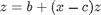
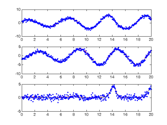
Smooth the data
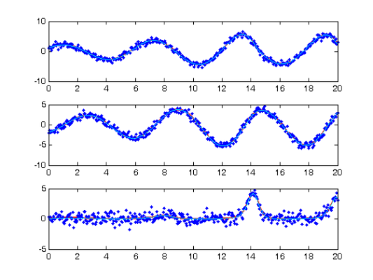
DEfd = smoothfd_cell(noise_path,tspan,Lfd_cell);
coefs = getcellcoefs(DEfd);

devals = eval_fdcell(tfine,DEfd,0);
for(i = 1:length(path))
    subplot(length(path),1,i);
    plot(tfine,devals{i},'r','LineWidth',2);
    hold on;
    plot(tspan{i},noise_path{i},'b.');
    hold off;
end
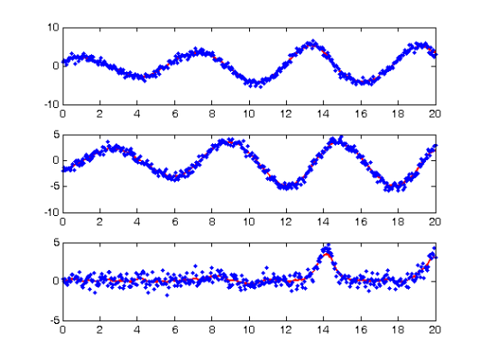
Re-smoothing with model-based penalty
% Call the Gauss-Newton solver

[newcoefs,resnorm2] = lsqnonlin(@SplineCoefErr,coefs,...
    [],[],lsopts_other,basis_cell,noise_path,tspan,wts,lambda,fn,...
    dfdy,[],[],[],ppars);

tDEfd = Make_fdcell(newcoefs,basis_cell);

% Plot results along with exact solution

devals = eval_fdcell(tfine,tDEfd,0);
for(i = 1:length(path))
    subplot(length(path),1,i);
    plot(tfine,devals{i},'r','LineWidth',2);
    hold on;
    plot(tspan{i},noise_path{i},'b.');
    plot(plot_time,plot_path(:,i),'c');
    hold off
end
                                         Norm of      First-order
 Iteration  Func-count     f(x)          step          optimality   CG-iterations
     0          1          229369                     1.57e+004
     1          2         12060.1        4.99116       1.6e+003           14
     2          3         4973.78             10      1.51e+003          165
     3          4         1151.34        13.1452            937          160
     4          5         812.383        0.33509           37.6           26
     5          6         812.383        10.8313           37.6          306
     6          7         732.104        2.70784            206            0
     7          8         732.104        5.41567            206          215
     8          9         685.263        1.35392            385            0
     9         10         660.713        2.70784            226          222
    10         11         625.084      0.0555431           25.8           11
    11         12         622.832        2.70784            214          294
    12         13         601.016      0.0392269             26           10
    13         14         598.501       0.676959           29.7          292
    14         15         597.705       0.570007           22.6          250
    15         16         597.652     0.00227555          0.993           13
    16         17         597.609       0.198483           15.9          416
    17         18         597.606    0.000391115          0.371           10
    18         19         597.605      0.0336477          0.107          556
    19         20         597.605     0.00760102        0.00435          508
    20         21         597.605     0.00188402        0.00225          547
    21         22         597.605     0.00040236      6.65e-005          524
    22         23         597.605     0.00011288       0.000161          555
    23         24         597.605   2.54135e-005      1.63e-005          558
    24         25         597.605   7.69495e-006      1.26e-005          550
    25         26         597.605   1.79362e-006      2.18e-006          396
Optimization terminated: relative function value
 changing by less than OPTIONS.TolFun.
Perform the Profiled Estimation
[newpars,newDEfd_cell] = Profile_GausNewt(ppars,lsopts_out,DEfd,fn,...
    dfdy,dfdp,d2fdy2,d2fdydp,lambda,noise_path,tspan,wts,...
    [],[],[],[],lsopts_in);

disp(newpars);
 Iteration       steps    Residual   Improvement   Grad-norm     parameters
     1           1         256.672      0.513038          265     0.1563     0.26934      3.0183
     2           1         198.494      0.226661         12.5     0.19974      0.2008      2.9388
     3           1         197.588    0.00456608        0.695     0.19932     0.20653       3.034
     4           1         197.587  4.43208e-006      0.00502     0.19943       0.206      3.0335
     5           1         197.587  6.47181e-009      0.00083     0.19943     0.20604      3.0337
    0.1994
    0.2060
    3.0337
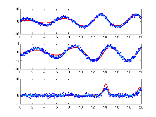
Plot Smooth with Profile-Estimated Parameters
devals = eval_fdcell(tfine,newDEfd_cell,0);
for(i = 1:length(path))
    subplot(length(path),1,i)
    plot(tfine,devals{i},'r','LineWidth',2);
    hold on;
    plot(tspan{i},noise_path{i},'b.');
    plot(plot_time,plot_path(:,i),'c');
    hold off
end
Comparison with Smooth Using True Parameters
coefs = getcellcoefs(DEfd);   % Starting coefficient estimates

[truecoefs,resnorm4] = lsqnonlin(@SplineCoefErr,coefs,[],[],...
    lsopts_other,basis_cell,noise_path,tspan,wts,lambda,fn,dfdy,...
    [],[],[],pars);

trueDEfd_cell = Make_fdcell(truecoefs,basis_cell);

devals = eval_fdcell(tfine,trueDEfd_cell,0);
for(i = 1:length(path))
    subplot(length(path),1,i)
    plot(plot_time,plot_path(:,i),'c')
    plot(tfine,devals{i},'r','LineWidth',2);
    hold on;
    plot(plot_time,plot_path(:,i),'c');
    plot(tspan{i},noise_path{i},'b.');
    hold off;
end
                                         Norm of      First-order
 Iteration  Func-count     f(x)          step          optimality   CG-iterations
     0          1          199278                     1.83e+004
     1          2         4085.02        3.58379      1.01e+003           10
     2          3         377.193        2.49177            232           38
     3          4         220.163        2.33239            129          140
     4          5         214.834        2.92018            747          301
     5          6         199.351      0.0321855             18           13
     6          7         198.667       0.477268           8.21          327
     7          8           198.5       0.505036           17.4          515
     8          9          198.49    0.000870897          0.338           14
     9         10         198.489     0.00713026         0.0203          221
    10         11         198.489      0.0119639        0.00803          541
    11         12         198.489    0.000835713       0.000177          448
    12         13         198.489    0.000191154         0.0001          603
    13         14         198.489   9.78293e-007      4.89e-006           48
    14         15         198.489   4.39558e-006       1.9e-006          603
    15         16         198.489   2.58483e-009      4.11e-007           21
Optimization terminated: relative function value
 changing by less than OPTIONS.TolFun.
Squared Error Performance
% Squared error for estimated parameters

newpreds = eval_fdcell(tspan,newDEfd_cell,0);
new_err = cell(length(newpreds));
for(i = 1:length(path))
    new_err{i} = wts(i)*(newpreds{i} - noise_path{i}).^2;
end

new_err = mean(cell2mat(new_err));

% Squared error for true parameters

truepreds = eval_fdcell(tspan,trueDEfd_cell,0);
true_err = cell(length(truepreds));
for(i = 1:length(path))
    true_err{i} = wts(i)*(truepreds{i} - noise_path{i}).^2;
end

true_err = mean(cell2mat(true_err));

% print out a comparsion

disp([new_err true_err]);
0.1642 0.1643
Calculate Sample Information and Variance-Covariance Matrices
% Hessian of squared error with respect to parameters

d2Jdp2 = make_d2jdp2(newDEfd_cell,fn,dfdy,dfdp,d2fdy2,d2fdydp,d2fdp2,...
    d3fdy3,d3fdy2dp,d3fdydp2,tspan,lambda,newpars,[],wts,...
    [],[],[],noise_path)

% Second derivatives with respect to parameters and observations

d2JdpdY = make_d2jdpdy(newDEfd_cell,fn,dfdy,d2fdy2,d3fdy3,dfdp,d2fdydp,d3fdy2dp,...
    tspan,lambda,newpars,[],wts,[],[],[],noise_path);

% Resulting derivative of parameters with respect to observations

dpdY = -d2Jdp2\d2JdpdY;

% Variance of observations:

S = make_sigma(DEfd,tspan,noise_path,0);

% Resulting parameter covariance matrix:

Cov = dpdY*S*dpdY'
d2Jdp2 =

  1.0e+004 *

    3.4315   -0.4993   -0.0084
   -0.4993    0.4205   -0.0785
   -0.0084   -0.0785    0.0272


Cov =

    0.0000    0.0000    0.0002
    0.0000    0.0003    0.0009
    0.0002    0.0009    0.0037